
|
|||||||||||||||||||||||
|
Lecture 9
Page last edited by Andrea Cuttone (ancu) 01/04-2014
Learning objectives Today is the second part of our two-week course on dynamic networks
We will continue working with the Wikispeedia dataset that contains data on a condensed version of Wikipedia with 4604 articles, as well as information on surfing on that network. To visualize and analyze the network, we will use Gephi a free tool for nework visualization and analysis.
Exercises 1) Download Gephi, and work through the quick start guide so you get a feel for how the program works: Also, check out the video on community detection (modularity) and visualizationL 2) Start by creating a networkx DiGraph from paths_finished.tsv as you did for Week 8 Exercise 2/3. Make sure to store the edge weights as ‘weight’ attribute on each edge. Export the graph to graphml with nx.write_graphml.
Visualize the network and an aspect of the dynamics. Since this is the last lecture, you're ready for a more free assignment, so the details are up to you! But make sure that you explain the thoughts you have put into the visualization.
We note that this network is difficult to visualize because it's so dense. For that reason we have created a little exploration of the network so you have a place to start from ... and you can explore some of the possibilities. (Thus, it's recommended that you work through the example below).
An example nework visualization
a) Go to Tools > Plugin menu > Available Plugins
> Check For Updates > Search for “circular” > select
Circular Layout > Install
b) Open the graphml file in
Gephi. Select Circular
Layout > Run
 c) We can filter out the low degree edges, using the following
command. Filters >
Topology > Degree range > choose 75 as lower bound >
Filter. And we can plot the resulting graph
Layout > Force Atlas > Check
Attraction Distribution and Adjust by Size >
Run
 d) Now, let's see the node names Select Ranking > Nodes > Size/Weight
button / Degree > Apply. Then Enable text
 e) And we can find communities (groups of densely connected
nodes) in the network. Start with Statistics > Modularity >
Run. Now, let's see
it on the network: Partition > Refresh button >
Modularity class > Apply
 f) Let's see the network in a circle ... and order the
circle by community. Circle layout > Order : Modularity
class
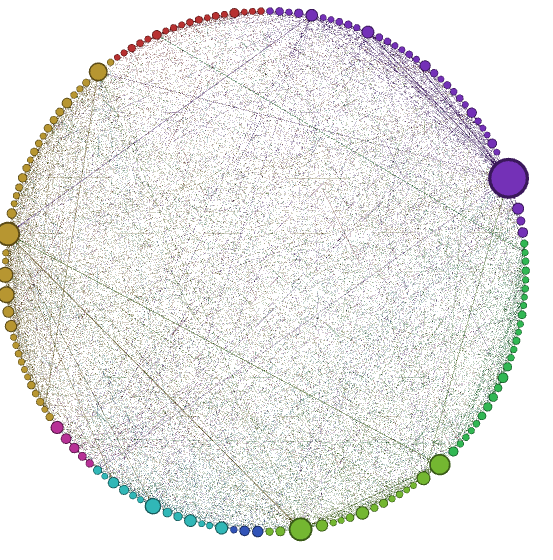 g) A great way of simplifying dense networks is by extrating
the multi-scale
backbone [
code here]. Try different values for the alpha parameter.
Repeat previous steps to create
new versions of the graphs and repeat the analysis.
  h) And you can try
different settings for filtering, layout algorithms, nodes
sizes
i) And take different time slices of the graphs and
compare the results
|
||||||||||||||||||||||

